Detecting Anomalies in Social Media Volume Time Series | by Lorenzo Mezzini | Nov, 2024

Analyzing a Sample Twitter Volume Dataset

Let’s start by loading and visualizing a sample Twitter volume dataset for Apple:

From this plot, we can see that there are several spikes (anomalies) in our data. These spikes in volumes are the ones we want to identify.

Looking at the second plot (log-scale) we can see that the Twitter volume data shows a clear daily cycle, with higher activity during the day and lower activity at night. This seasonal pattern is common in social media data, as it reflects the day-night activity of users. It also presents a weekly seasonality, but we will ignore it.

Removing Seasonal Trends

We want to make sure that this cycle does not interfere with our conclusions, thus we will remove it. To remove this seasonality, we’ll perform a seasonal decomposition.

First, we’ll calculate the moving average (MA) of the volume, which will capture the trend. Then, we’ll compute the ratio of the observed volume to the MA, which gives us the multiplicative seasonal effect.

As expected, the seasonal trend follows a day/night cycle with its peak during the day hours and its saddle at nighttime.

To further proceed with the decomposition we need to calculate the expected value of the volume given the multiplicative trend found before.

Analyzing Residuals and Detecting Anomalies

The final component of the decomposition is the error resulting from the subtraction between the expected value and the true value. We can consider this measure as the de-meaned volume accounting for seasonality:

Interestingly, the residual distribution closely follows a Pareto distribution. This property allows us to use the Pareto distribution to set a threshold for detecting anomalies, as we can flag any residuals that fall above a certain percentile (e.g., 0.9995) as potential anomalies.

Now, I have to do a big disclaimer: this property I am talking about is not “True” per se. In my experience in social listening, I’ve observed that holds true with most social data. Except for some right skewness in a dataset with many anomalies.

In this specific case, we have well over 15k observations, hence we will set the p-value at 0.9995. Given this threshold, roughly 5 anomalies for every 10.000 observations will be detected (assuming a perfect Pareto distribution).

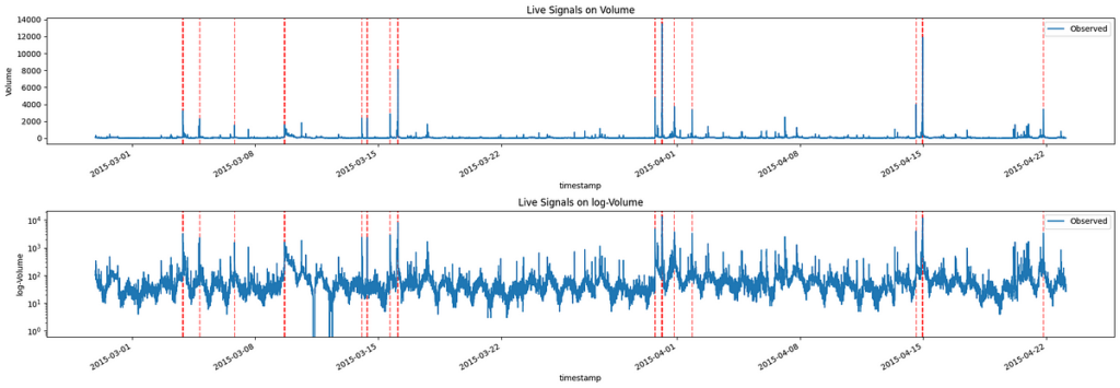
Therefore, if we check which observation in our data has an error whose p-value is higher than 0.9995, we get the following signals:

From this graph, we see that the observations with the highest volumes are highlighted as anomalies. Of course, if we desire more or fewer signals, we can adjust the selected p-value, keeping in mind that, as it decreases, it will increase the number of signals.