Learn Transformer Fine-Tuning and Segment Anything | by Stefan Todoran | Jun, 2024

Train Meta’s Segment Anything Model (SAM) to segment high fidelity masks for any domain

The release of several powerful, open-source foundational models coupled with advancements in fine-tuning have brought about a new paradigm in machine learning and artificial intelligence. At the center of this revolution is the transformer model.

While high accuracy domain-specific models were once out of reach for all but the most well funded corporations, today the foundational model paradigm allows for even the modest resources available to student or independent researchers to achieve results rivaling state of the art proprietary models.

This article explores the application of Meta’s Segment Anything Model (SAM) to the remote sensing task of river pixel segmentation. If you’d like to jump right in to the code the source file for this project is available on GitHub and the data is on HuggingFace, although reading the full article first is advised.

The first step is to either find or create a suitable dataset. Based on existing literature, a good fine-tuning dataset for SAM will have at least 200–800 images. A key lesson of the past decade of deep learning advancement is that more data is always better, so you can’t go wrong with a larger fine-tuning dataset. However, the goal behind foundational models is to allow even relatively small datasets to be sufficient for strong performance.

It will also be necessary to have a HuggingFace account, which can be created here. Using HuggingFace we can easily store and fetch our dataset at any time from any device, which makes collaboration and reproducibility easier.

The last requirement is a device with a GPU on which we can run the training workflow. An Nvidia T4 GPU, which is available for free through Google Colab, is sufficiently powerful to train the largest SAM model checkpoint (sam-vit-huge) on 1000 images for 50 epochs in under 12 hours.

To avoid losing progress to usage limits on hosted runtimes, you can mount Google Drive and save each model checkpoint there. Alternatively, deploy and connect to a GCP virtual machine to bypass limits altogether. If you’ve never used GCP before you are eligible for a free $300 dollar credit, which is enough to train the model at least a dozen times.

Before we begin training, we need to understand the architecture of SAM. The model contains three components: an image encoder from a minimally modified masked autoencoder, a flexible prompt encoder capable of processing diverse prompt types, and a quick and lightweight mask decoder. One motivation behind the design is to allow fast, real-time segmentation on edge devices (e.g. in the browser) since the image embedding only needs to be computed once and the mask decoder can run in ~50ms on CPU.

In theory, the image encoder has already learned the optimal way to embed an image, identifying shapes, edges and other general visual features. Similarly, in theory the prompt encoder is already able to optimally encode prompts. The mask decoder is the part of the model architecture which takes these image and prompt embeddings and actually creates the mask by operating on the image and prompt embeddings.

As such, one approach is to freeze the model parameters associated with the image and prompt encoders during training and to only update the mask decoder weights. This approach has the benefit of allowing both supervised and unsupervised downstream tasks, since control point and bounding box prompts are both automatable and usable by humans.

An alternative approach is to overload the prompt encoder, freezing the image encoder and mask decoder and simply not using the original SAM mask encoder. For example, the AutoSAM architecture uses a network based on Harmonic Dense Net to produce prompt embeddings based on the image itself. In this tutorial we will cover the first approach, freezing the image and prompt encoders and training only the mask decoder, but code for this alternative approach can be found in the AutoSAM GitHub and paper.

The next step is to determine what sorts of prompts the model will receive during inference time, so that we can supply that type of prompt at training time. Personally I would not advise the use of text prompts for any serious computer vision pipeline, given the unpredictable/inconsistent nature of natural language processing. This leaves points and bounding boxes, with the choice ultimately being down to the particular nature of your specific dataset, although the literature has found that bounding boxes outperform control points fairly consistently.

The reasons for this are not entirely clear, but it could be any of the following factors, or some combination of them:

• Good control points are more difficult to select at inference time (when the ground truth mask is unknown) than bounding boxes.
• The space of possible point prompts is orders of magnitude larger than the space of possible bounding box prompts, so it has not been as thoroughly trained.
• The original SAM authors focused on the model’s zero-shot and few-shot (counted in term of human prompt interactions) capabilities, so pretraining may have focused more on bounding boxes.

Regardless, river segmentation is actually a rare case in which point prompts actually outperform bounding boxes (although only slightly, even with an extremely favorable domain). Given that in any image of a river the body of water will stretch from one end of the image to another, any encompassing bounding box will almost always cover most of the image. Therefore the bounding box prompts for very different portions of river can look extremely similar, in theory meaning that bounding boxes provide the model with significantly less information than control points and therefore leading to worse performance.

Notice how in the illustration above, although the true segmentation masks for the two river portions are completely different, their respective bounding boxes are nearly identical, while their points prompts differ (comparatively) more.

The other important factor to consider is how easily input prompts can be generated at inference time. If you expect to have a human in the loop, then both bounding boxes and control points are both fairly trivial to acquire at inference time. However in the event that you intend to have a completely automated pipeline, answering this questions becomes more involved.

Whether using control points or bounding boxes, generating the prompt typically first involves estimating a rough mask for the object of interest. Bounding boxes can then just be the minimum box which wraps the rough mask, whereas control points need to be sampled from the rough mask. This means that bounding boxes are easier to obtain when the ground truth mask is unknown, since the estimated mask for the object of interest only needs to roughly match the same size and position of the true object, whereas for control points the estimated mask would need to more closely match the contours of the object.

For river segmentation, if we have access to both RGB and NIR, then we can use spectral indices thresholding methods to obtain our rough mask. If we only have access to RGB, we can convert the image to HSV and threshold all pixels within a certain hue, saturation, and value range. Then, we can remove connected components below a certain size threshold and use erosion from skimage.morphology to make sure the only 1 pixels in our mask are those which were towards the center of large blue blobs.

To train our model, we need a data loader containing all of our training data that we can iterate over for each training epoch. When we load our dataset from HuggingFace, it takes the form of a datasets.Dataset class. If the dataset is private, make sure to first install the HuggingFace CLI and sign in using !huggingface-cli login.

from datasets import load_dataset, load_from_disk, Dataset
hf_dataset_name = "stodoran/elwha-segmentation-v1"
training_data = load_dataset(hf_dataset_name, split="train")
validation_data = load_dataset(hf_dataset_name, split="validation")

We then need to code up our own custom dataset class which returns not just an image and label for any index, but also the prompt. Below is an implementation that can handle both control point and bounding box prompts. To be initialized, it takes a HuggingFace datasets.Dataset instance and a SAM processor instance.

from torch.utils.data import Dataset
class PromptType:
CONTROL_POINTS = "pts"
BOUNDING_BOX = "bbox"
class SAMDataset(Dataset):
def __init__(
self, 
dataset, 
processor, 
prompt_type = PromptType.CONTROL_POINTS,
num_positive = 3,
num_negative = 0,
erode = True,
multi_mask = "mean",
perturbation = 10,
image_size = (1024, 1024),
mask_size = (256, 256),
):
# Asign all values to self
...
def __len__(self):
return len(self.dataset)
def __getitem__(self, idx):
datapoint = self.dataset[idx]
input_image = cv2.resize(np.array(datapoint["image"]), self.image_size)
ground_truth_mask = cv2.resize(np.array(datapoint["label"]), self.mask_size)
if self.prompt_type == PromptType.CONTROL_POINTS:
inputs = self._getitem_ctrlpts(input_image, ground_truth_mask)
elif self.prompt_type == PromptType.BOUNDING_BOX:
inputs = self._getitem_bbox(input_image, ground_truth_mask)
inputs["ground_truth_mask"] = ground_truth_mask
return inputs

We also have to define the SAMDataset._getitem_ctrlpts and SAMDataset._getitem_bbox functions, although if you only plan to use one prompt type then you can refactor the code to just directly handle that type in SAMDataset.__getitem__ and remove the helper function.

class SAMDataset(Dataset):
...
def _getitem_ctrlpts(self, input_image, ground_truth_mask):
# Get control points prompt. See the GitHub for the source
# of this function, or replace with your own point selection algorithm.
input_points, input_labels = generate_input_points(
num_positive=self.num_positive,
num_negative=self.num_negative,
mask=ground_truth_mask,
dynamic_distance=True,
erode=self.erode,
)
input_points = input_points.astype(float).tolist()
input_labels = input_labels.tolist()
input_labels = [[x] for x in input_labels]
# Prepare the image and prompt for the model.
inputs = self.processor(
input_image,
input_points=input_points,
input_labels=input_labels,
return_tensors="pt"
)
# Remove batch dimension which the processor adds by default.
inputs = {k: v.squeeze(0) for k, v in inputs.items()}
inputs["input_labels"] = inputs["input_labels"].squeeze(1)
return inputs
def _getitem_bbox(self, input_image, ground_truth_mask):
# Get bounding box prompt.
bbox = get_input_bbox(ground_truth_mask, perturbation=self.perturbation)
# Prepare the image and prompt for the model.
inputs = self.processor(input_image, input_boxes=[[bbox]], return_tensors="pt")
inputs = {k: v.squeeze(0) for k, v in inputs.items()} # Remove batch dimension which the processor adds by default.
return inputs

Putting it all together, we can create a function which creates and returns a PyTorch dataloader given either split of the HuggingFace dataset. Writing functions which return dataloaders rather than just executing cells with the same code is not only good practice for writing flexible and maintainable code, but is also necessary if you plan to use HuggingFace Accelerate to run distributed training.

from transformers import SamProcessor
from torch.utils.data import DataLoader
def get_dataloader(
hf_dataset,
model_size = "base",  # One of "base", "large", or "huge" 
batch_size = 8, 
prompt_type = PromptType.CONTROL_POINTS,
num_positive = 3,
num_negative = 0,
erode = True,
multi_mask = "mean",
perturbation = 10,
image_size = (256, 256),
mask_size = (256, 256),
):
processor = SamProcessor.from_pretrained(f"facebook/sam-vit-{model_size}")
sam_dataset = SAMDataset(
dataset=hf_dataset, 
processor=processor, 
prompt_type=prompt_type,
num_positive=num_positive,
num_negative=num_negative,
erode=erode,
multi_mask=multi_mask,
perturbation=perturbation,
image_size=image_size,
mask_size=mask_size,
)
dataloader = DataLoader(sam_dataset, batch_size=batch_size, shuffle=True)
return dataloader

After this, training is simply a matter of loading the model, freezing the image and prompt encoders, and training for the desired number of iterations.

model = SamModel.from_pretrained(f"facebook/sam-vit-{model_size}")
optimizer = AdamW(model.mask_decoder.parameters(), lr=learning_rate, weight_decay=weight_decay)
# Train only the decoder.
for name, param in model.named_parameters():
if name.startswith("vision_encoder") or name.startswith("prompt_encoder"):
param.requires_grad_(False)

Below is the basic outline of the training loop code. Note that the forward_pass, calculate loss, evaluate_model, and save_model_checkpoint functions have been left out for brevity, but implementations are available on the GitHub. The forward pass code will differ slightly based on the prompt type, and the loss calculation needs a special case based on prompt type as well; when using point prompts, SAM returns a predicted mask for every single input point, so in order to get a single mask which can be compared to the ground truth either the predicted masks need to be averaged, or the best predicted mask needs to be selected (identified based on SAM’s predicted IoU scores).

train_losses = []
validation_losses = []
epoch_loop = tqdm(total=num_epochs, position=epoch, leave=False)
batch_loop = tqdm(total=len(train_dataloader), position=0, leave=True)
while epoch < num_epochs:
epoch_losses = []
batch_loop.n = 0  # Loop Reset
for idx, batch in enumerate(train_dataloader):
# Forward Pass
batch = {k: v.to(accelerator.device) for k, v in batch.items()}
outputs = forward_pass(model, batch, prompt_type)
# Compute Loss
ground_truth_masks = batch["ground_truth_mask"].float()
train_loss = calculate_loss(outputs, ground_truth_masks, prompt_type, loss_fn, multi_mask="best")
epoch_losses.append(train_loss)
# Backward Pass & Optimizer Step
optimizer.zero_grad()
accelerator.backward(train_loss)
optimizer.step()
lr_scheduler.step()
batch_loop.set_description(f"Train Loss: {train_loss.item():.4f}")
batch_loop.update(1)
validation_loss = evaluate_model(model, validation_dataloader, accelerator.device, loss_fn)
train_losses.append(torch.mean(torch.Tensor(epoch_losses)))
validation_losses.append(validation_loss)
if validation_loss < best_loss:
save_model_checkpoint(
accelerator,
best_checkpoint_path,
model,
optimizer,
lr_scheduler,
epoch,
train_history,
validation_loss,
train_losses,
validation_losses,
loss_config,
model_descriptor=model_descriptor,
)
best_loss = validation_loss
epoch_loop.set_description(f"Best Loss: {best_loss:.4f}")
epoch_loop.update(1)
epoch += 1

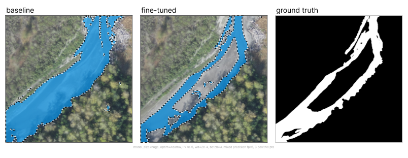
For the Elwha river project, the best setup achieved trained the “sam-vit-base” model using a dataset of over 1k segmentation masks using a GCP instance in under 12 hours.

Compared with baseline SAM the fine-tuning drastically improved performance, with the median mask going from unusable to highly accurate.

One important fact to note is that the training dataset of 1k river images was imperfect, with segmentation labels varying greatly in the amount of correctly classified pixels. As such, the metrics shown above were calculated on a held-out pixel perfect dataset of 225 river images.

An interesting observed behavior was that the model learned to generalize from the imperfect training data. When evaluating on datapoints where the training example contained obvious misclassifications, we can observe that the models prediction avoids the error. Notice how images in the top row which shows training samples contains masks which do not fill the river in all the way to the bank, while the bottom row showing model predictions more tightly segments river boundaries.